
 Open Access Article
 This Open Access Article is licensed under a
 Creative Commons Attribution 3.0 Unported Licence
Vibrationally resolved optical spectra of modified diamondoids obtained from time-dependent correlation function methods
Shiladitya
Banerjee
,
Tony
Stüker
and
Peter
Saalfrank
*
Institut für Chemie, Universität Potsdam, Karl-Liebknecht-Straße 24-25, D-14476 Potsdam-Golm, Germany. E-mail: peter.saalfrank@uni-potsdam.de
First published on the web 1st July 2015
Optical properties of modified diamondoids have been studied theoretically using vibrationally resolved electronic absorption, emission and resonance Raman spectra. A time-dependent correlation function approach has been used for electronic two-state models, comprising a ground state (g) and a bright, excited state (e), the latter determined from linear-response, time-dependent density functional theory (TD-DFT). The harmonic and Condon approximations were adopted. In most cases origin shifts, frequency alteration and Duschinsky rotation in excited states were considered. For other cases where no excited state geometry optimization and normal mode analysis were possible or desired, a short-time approximation was used. The optical properties and spectra have been computed for (i) a set of recently synthesized sp2/sp3 hybrid species with C![[double bond, length as m-dash]](../../../../../../www.rsc.org/images/entities/char_e001.gif) C double-bond connected saturated diamondoid subunits, (ii) functionalized (mostly by thiol or thione groups) diamondoids and (iii) urotropine and other C-substituted diamondoids. The ultimate goal is to tailor optical and electronic features of diamondoids by electronic blending, functionalization and substitution, based on a molecular-level understanding of the ongoing photophysics.
C double-bond connected saturated diamondoid subunits, (ii) functionalized (mostly by thiol or thione groups) diamondoids and (iii) urotropine and other C-substituted diamondoids. The ultimate goal is to tailor optical and electronic features of diamondoids by electronic blending, functionalization and substitution, based on a molecular-level understanding of the ongoing photophysics.
I. Introduction
Diamondoids form a family of hydrocarbons, consisting of repeated units of connected cyclohexane rings.1–3 The first member of this series is adamantane, C10H16, a saturated diamondoid with sp3-hybridized carbon atoms. Higher homologues are known as diamantane, C14H20, triamantane C18H24, tetramantane C22H28, pentamantane and so on. Diamondoids are chemically quite inert, hard compounds.4 They are good (monochromatic) electron emitters with negative electron affinity,5–7 transparent wide-gap materials, absorbing light significantly around and above about 6 eV,8–10i.e., in the UV. Diamondoids are excellent fluorescing materials, known to fluoresce both in the solid state and in the gas phase. For absorption to and fluorescence from, the lowest electronic excited states, often pronounced vibrational finestructures in spectra have been observed.10 Vibrations involving excited states are also important for the interpretation of resonance Raman spectra, another important tool to characterize diamondoids.11 In general, vibronic spectra are powerful tools to unravel details of optical properties of diamondoids and the focus of this paper.Due to the diverseness of their shape and composition and the ability to be functionalized (see below), one hopes that diamondoids have tunable optical and electronic properties for possible applications. Ref. 12 reported the effects of C–H and interstitial substitution on the HOMO–LUMO energy and the band gaps of a range of diamondoids, using density functional theory computations. Along these lines, the synthesis of artificial diamondoids has greatly advanced in recent years,13 as well as their spectroscopic investigation.14–18 The modified diamondoids studied in these works can roughly be classified according to three main categories:
(i) “Electronically blended diamondoids”, i.e., diamondoid subunits connected to each other by sp2-hybridized C atoms (or other unsaturated units). The subunits may be comprised of the same (DiaDia, two diamantanes; AdaAda, two adamantanes) or different (AdaDia, AdaDiaAda) diamondoid molecules. Several of these (and related) molecules have been synthesized by Schreiner and co-workers.11,13 For example, DiaDia which exists as E and Z stereoisomers has been the subject of recent physico-chemical11 and theoretical18 characterization. In DiaDia, a greatly reduced HOMO–LUMO gap is found compared to pristine diamondoids, as well as a strongly enhanced CC vibration in resonance Raman. Among other experimental studies, the valence photoelectron spectra of selected diamondoids, joined by single or double CC bonds have been measured in the recent past.19
To extend this work and identify trends in CC-blended diamondoids, other and also more complicated species such as AdaDiaAda (with two CC double bonds) will be considered here.
(ii) “Functionalized diamondoids”,15–17i.e., species where one or multiple H atom(s) were substituted by particular functional groups like hydroxyl, cyano, amino, or thiol (–SH) groups. Sulfur-containing diamondoids are particularly interesting because of the ease of their attachment to metal surfaces; their synthesis dates back nearly to a decade.20,21 It is possible to attach multiple functional groups, resulting in, e.g., dithiol, trithiol, and so on. Structural isomers also exist, depending on the position of the functional group (e.g., adamantane-1-thiol and adamantane-2-thiol) or the relative positions of two or more functional groups (e.g., adamantane-1,2-dithiol and adamantane-1,3-dithiol). Recently, Landt and co-workers showed that the incorporation of a thiol group in adamantane lowers its optical gap.15 This opens up the speculation on tunable optical properties of diamondoids by thiolization.
To identify trends in mono- vs. di-substitution as well as effects of the position of the functional group(s), on the optical gaps and the vibronic absorption, emission and resonance Raman spectra, various thiol- and dithiol-adamantanes will be studied in this work.
Also, the substitution (of two H atoms) by S groups, leading to thiones, e.g. adamantane thione, C10H14S, have been discussed in the literature as possible routes towards “tuned” materials. In a recent theoretical work,22 Vörös and co-workers predicted by PBE0/cc-pVTZ calculations for adamantane and [1(2,3)4]-pentamantane, that the optical gap is reduced gradually by the systematic substitution of thione groups. For adamantane-1,2,5,6-tetrathione and adamantane hexathione, for example, the optical gap was estimated to be in the visible range, between 2–3 eV.
No vibronic effects and real spectra were considered in that work, however, which we will do here for selected thionized diamondoids.
As a sideline, also several adamantanes functionalized with alcohol (–OH) and bromo (–Br) groups will be studied.
(iii) “Doping” or “C-substituting” diamondoids”, i.e., replacing one or more methine (CH) or methylene (CH2) groups of pristine diamondoids by iso-electronic groups such as N and O, is the final route of tuning properties of diamondoids to be studied here. This can lead to the formation of molecules with entirely new electronic and optical properties. For instance, substitution of the four –CH groups of adamantane by the iso-electronic N atom results in urotropine or hexamethylene tetramine, (CH2)6N4. In ref. 14, experiment has shown that the absorption and fluorescence of urotropine are very distinct from those of adamantane, with a “smooth”, redshifted absorption band with no pronounced vibrational finestructure.
In the present work, we shall study some of the photophysical properties of urotropine by electronic structure methods, as well as of several other N- or O-substituted adamantanes.
Our work focuses on comparing vibrationally resolved absorption, emission and resonance Raman (rR) spectra of representative diamondoids from each of the three categories mentioned, using a two-state model with the ground state (g, or S0) and one bright, excited state (e, usually S1). In certain cases also a wider range of excited states was considered, then, however, mostly only for vertical electronic excitation energies. The ground and excited states are calculated by hybrid density functional theory (DFT) and linear-response time-dependent DFT (TD-DFT), respectively. Pristine diamondoids will be used as a reference. We shall also compare to experiment where possible. Our ultimate goal is to understand the photophysics of modified diamondoids on a fundamental level, and – based on this understanding – to help developing criteria for the “tuning” of optoelectronic properties of these versatile materials.
In order to arrive at vibrationally resolved spectra, we use a time-dependent correlation function approach as pioneered in chemical physics by Heller and co-workers.23,24 The time-dependent approach can offer computational advantages by avoiding the computation of Franck–Condon factors. In particular in the harmonic approximation which we use here, quasi-analytic expressions are available for auto- and cross-correlation functions. By combining (TD-)DFT with the correlation function approach in harmonic approximation, vibronically resolved spectra become available for medium-sized molecules with moderate computational effort and acceptable accuracy. The largest molecule treated here is AdaDiaAda, C34H44, with 228 normal modes. Other diamondoids have been studied elsewhere with the same methodology18 and bigger molecules of different type, e.g., β-carotene (C40H56), in ref. 25. In that reference, also the inclusion of Duschinsky rotation for resonance Raman spectra when calculated with time-dependent correlation functions has been put forward. (The further extension of the time-dependent approach to Herzberg–Teller corrections for resonance Raman was realized in ref. 26 and 27.) Duschinksy rotation, i.e., the rotation of normal modes in the electronically excited state relative to ground state modes, is an effect which will be considered here in many but not all examples.
The paper is organized as follows. The methods, models and approximations used for the computation of the spectra are described in Section II. Results are presented and discussed in Section III, for electronically blended diamondoids (Section III A), thiol- and thione-substituted diamondoids (Section III B) and urotropine (Section III C). Section IV summarizes the work and provides an outlook for possible future investigations in this field.
II. Methods
The vibrationally resolved absorption, emission and resonance Raman spectra have been calculated using the time-dependent correlation function approach, as popularized by Heller and co-workers.23,24 Here we work in harmonic and Condon approximations, using two-state models. Normal-mode coordinates are used throughout (rather than curvilinear coordinates, which can lead to somewhat different results28), the temperature is 0 K and possible effects of an environment are neglected.In a first, more sophisticated model, called here the IMDHOFAD (independent mode displaced harmonic oscillator with frequency alteration and Duschinsky rotation) method, full geometry optimizations are carried out for the ground (g) and the selected bright, electronically excited state (e) and normal mode analyses are performed for both. Frequency alterations in the excited state and the Duschinsky rotation are taken fully into account. The method is described in more detail in ref. 18 and 25 and therefore only briefly reiterated below. In situations where optimization of excited states is not so trivial, unphysical, or simply unwanted (in order to save computational effort and allow for screening many molecules), the IMDHO (STA) approach will be used instead. In this approach,29 frequency alteration and Duschinsky rotation are not accounted for, and in addition the “short-time approximation” (STA) is used. Excited-state displacements are obtained from a local extrapolation scheme.
The first approach of above which is based on two fully optimized harmonic potentials, belongs to a broader class of models called “adiabatic”. The latter approach, on the other hand, belongs to so-called “vertical” methods for which only information (on gradients and/or Hessians) at a Franck–Condon point for vertical transitions between two potentials enters. The vertical approach is not only more economic as it avoids excited-state optimizations, it can also be of advantage if the excited state optimization is difficult, for practical or principal reasons, and then it is sometimes physically also more sensible. This is particularly so when large-amplitude motions and/or geometry displacements in excited states take place.28
For the adiabatic, IMDHOFAD model optimizations and normal mode analyses have been performed using density functional theory (DFT) and linear-response, time-dependent DFT (TD-DFT). Specifically, the B3LYP hybrid functional30,31 together with a triple zeta valence polarized (TZVP,32) basis set has been used throughout, if not explicitly stated otherwise. The validity of this method for diamondoids (good ratio of accuracy and computational effort), has been proven in ref. 18. The GAUSSIAN0933 quantum chemistry package has been used for optimizations and normal mode analyses. A FORTRAN code developed earlier25 was used to calculate the Duschinsky matrix and the dimensionless origin shifts between the normal modes of the two electronic states. The code is then used to calculate the auto-correlation functions and cross-correlation functions using the time-dependent approach. Spectra are obtained from Fourier transformed correlation functions by using the FFTW (Fastest Fourier Transform in the West) package.34 The IMDHO (STA) calculations, on the other hand, have been carried out directly with the quantum chemical package ORCA,35 on the (TD-)B3LYP/TZVP level of theory as well.
In the time-domain, the absorption cross-section is expressed as a Fourier transform of an autocorrelation function (we use atomic units in what follows)18,23
 | (1) |
 the transition dipole moment between g and e states, which is taken constant and equal to the value at the equilibrium geometry (0g) of the ground state, in the Condon approximation. Further, |ϕg0(0)〉 is a product vibrational, initial wavefunction comprising 3N − 6 vibrational ground state normal modes of the electronic ground state (N is the number of atoms). Γ is the width (of the Lorentzian) used for damping the autocorrelation function, 〈ϕg0(0)|e−iĤetϕg0(0)〉. Ĥe is the field-free, excited state nuclear Hamiltonian. In the harmonic approximation (even in the IMDHOFAD model), the expressions for multi-dimensional autocorrelation functions can be obtained analytically.23,25 Their computation requires optimized geometries of ground and excited states, ground and excited state normal frequencies ωg1,ωg2,…,ωg3N−6;ωe1,ωe2,…,ωe3N−6 and corresponding normal modes and, derived from these quantities, the Duschinsky matrix and the so-called dimensionless origin shifts for modes.
The emission cross-section can also be expressed as the Fourier transform of a time-dependent correlation function
 | (2) |
 is the transition dipole moment, evaluated now at the optimized geometry of the excited state (0e). Like absorption, expressions for multi-dimensional autocorrelation functions can be obtained quasi-analytically.23,25
The resonance Raman (rR) cross-section is calculated using
 | (3) |
 is the Raman polarizability for rR scattering from vibrational level i to f, in the ground electronic state. For 0 → 1 Raman scattering as considered in this work, i = 0, f = 1. q and q′ refer to the x, y or z directions, along which the components of the transition dipole moment are considered. In the time-dependent regime, the Raman polarizability can be calculated as a Fourier transform of a cross-correlation function18,24
 | (4) |
 is usually adopted for rR spectra. Here we compute rR spectra by fixing the excitation wavelengths ωL at certain values close to electronic excitation energies, as a function of the Raman shift. For 0 → 1 Raman scattering, we then obtain a stick spectrum as a function of the ground state vibrational frequencies, which is broadened here by Lorentzians of appropriate FWHM.
As outlined above, the time-dependent approach offers a variant, the short-time approximation (STA) which can be applied for absorption, emission and rR intensities.24,29 As stated, the STA is not always an approximation but may, as a representative of the “vertical” models, in certain special situations be even more accurate than the full IMDHOFAD model. In the STA approach to absorption as implemented in ORCA,29 excited-state energies are calculated for a particular set of geometries at and around the ground state geometry and quadratic fits to these energies are used to estimate a harmonic excited surface without explicitly optimizing its geometry and performing a normal mode analysis. Rather, this method neglects frequency alterations and mode-mixing in the excited state and will therefore be referred to as the IMDHO (STA) approach in what follows. Specifically, mode displacements are calculated using the relation, for absorption29
 | (5) |
 is the gradient of the excited state potential energy Ve along the mth mass weighted normal coordinate of a ground state mode, at the equilibrium geometry of the ground state (Franck–Condon point) and ωem is the excited state frequency of the mth normal mode. In the IMDHO model, excited state frequencies are assumed to be the same as the ground state frequencies ωgm. The dimensionless shift of the mth normal mode, Δm is then obtained from the relation
 | (6) |
III. Results
A. Electronically blended diamondoids
Let us first study molecules containing one or two CC double bonds which connect simple diamondoids, such as adamantane (Ada) or diamantane (Dia). Specifically, we consider AdaAda, AdaDia, DiaDia and AdaDiaAda, which are experimentally known.11 DiaDia exists as two geometric isomers, E and Z, depending on the geometry around the CC bond connecting the two diamantane units and has been studied with analogous theoretical models in ref. 18. Most optical and electronic properties of E and Z are very similar and so are their energies. For AdaAda and AdaDia no analogous isomers exist. Fig. 1 shows the optimized geometries in their ground electronic states for the two other diamondoids containing a single CC bond as studied here, namely AdaAda and AdaDia.
 | ||
| Fig. 1 The optimized geometries at the ground electronic states (S0, g) of AdaAda (a) and AdaDia (b), at the B3LYP/TZVP level of theory. Brown balls represent the C atoms and the white balls H atoms. The central bond joining the two diamondoid units is a CC double bond, with a bond length of 1.34 Å for either. Other C–C bonds are single, with bond lengths typically of 1.54 Å. The CC bond-length compares well with recently available experimental (1.34 Å for AdaAda and 1.33 Å for AdaDia) and theoretical (DFT and MP2) data.36 The calculated C–H bond lengths (1.09 Å) also show good agreement with the corresponding experimental data. | ||
Considering the lowest-energy, bright (S0 → S1) absorption transitions of DiaDia, AdaAda and AdaDia, we show in Table 1 the HOMO–LUMO gaps ΔEHL (calculated for Kohn–Sham orbital energies) and vertical excitation energies ΔEvert (calculated from TD-DFT) for these compounds. We also compare to the lowest-energy, bright transitions for adamantane.18
Dia(E) and DiaDia(Z) were already reported in ref. 18. Also values for Ada are shown, taken from the same reference
| Molecule | ΔEHL | ΔE0–0 | ΔEvert | ΔEvibro |
|---|---|---|---|---|
| Adamantane (Ada) | 8.15 | 6.54 | 7.32 | 6.84 |
| AdaAda |
6.34 | 5.20 | 5.60 | 5.48 |
| AdaDia |
6.28 | 5.16 | 5.55 | 5.44 |
| DiaDia(E) |
6.23 | 5.14 | 5.52 | 5.41 |
| DiaDia(Z) |
6.22 | 5.11 | 5.50 | 5.38 |
Considering Ada as a reference first, experimentally it is known that this parent compound has an optical gap (the onset of absorption) of 6.49 eV,10 which is close to the experimental 0–0 transition in this case (see also Table 6 below). (The optical gap of Dia is found to be 6.40 eV according to that ref. 10.) From Table 1 we see that the theoretical ΔE0–0 value is close to the experimental one. The vertical excitation energy is 7.32 eV for adamantane and unknown experimentally. From the table it is seen that the energy gaps decrease considerably when Ada/Dia subunits are connected by CC bonds. Taking ΔE0–0 values as a measure for optical gap reduction, the latter is in the order of 1.3 eV and close to up to about 2 eV if ΔEvert are considered (relative to Ada). Both the ΔE0–0 and ΔEvert values of AdaAda, DiaDia and AdaDia are all very similar (within ∼0.1 eV). The lowest allowed electronic transition to S1 for the electronically blended diamondoids involves a dominant HOMO → LUMO transition, which is relatively weak for AdaAda, AdaDia and also the previously studied DiaDia(E). For DiaDia(E) the vertical transition energy to S1 at ω1 = 5.52 eV has an oscillator strength of f1 = 0.00039.18 The HOMO is the CC π-orbital, and the LUMO is a diffuse orbital delocalized over the periphery of the molecule. A similar behavior is found for the species studied here, AdaAda and AdaDia. It should be noted that, due to relatively low oscillator strengths, the S1 state does not dominate the spectrum, however. Rather, the most intense transition is due to a CC π → π* excitation at higher energies. For DiaDia(E), for example, π* is the LUMO+2, which, like π, is strongly localized around the CC bond. The corresponding excited state is S4 in case of DiaDia(E), at a vertical transition energy of ω4 = 6.34 eV and an oscillator strength of f4 = 0.8327.18 (States S2 and S3 are dark states in case of DiaDia(E).)
Table 1 also demonstrates that ΔEHL values should not be considered as reliable estimates of optical gaps, being about 0.8 eV larger than ΔEvert. Another measure for optical excitations is the vibronic energy difference ΔEvibro, i.e., the maximum of the vibronically resolved absorption spectra. ΔEvibro is also listed in the table, showing similar (but slightly lower) values than ΔEvert. For the unsaturated species, ΔEvert is reduced by about 1.8 eV compared to a saturated diamondoid such as Ada. The strong reduction of the optical gap in CC-connected dimers by the here observed order of magnitude is very consistent with experimental findings.11
To illustrate effects of the vibronic finestructure on spectra in detail, we show in Fig. 2 absorption, emission and resonance Raman spectra for AdaAda and AdaDia, obtained by using (TD-)B3LYP/TZVP/IMDHOFAD and the S0 and S1 states. Let us consider the absorption and emission spectra (upper panels) first. For both molecules it is seen that indeed, the 0–0 transitions are not clearly visible either in absorption or in emission. This is because some modes exhibit very high values of adimensional shifts, up to 4 (compared to the usual values which lie around 1). All absorption and emission spectra show a pronounced vibrational finestructure. For both molecules, the maximal absorption peak is close to the vertical excitation energies, i.e., ΔEvert ∼ ΔEvibr as already demonstrated in Table 1 (both ΔE0–0 and ΔEvert are shown as dashed, vertical lines). As a fine detail, we note that the absorption and emission spectra of AdaDia (b) are slightly more structured than those of AdaAda (a), but are similar otherwise. Also the corresponding spectra of DiaDia (see Fig. 10 of ref. 18) look similar.
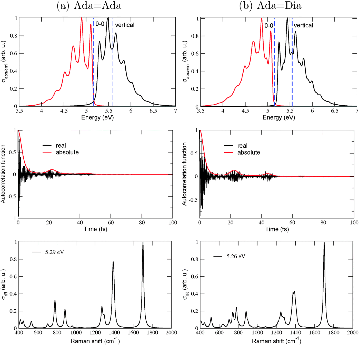 | ||
Fig. 2 The vibrationally resolved absorption, emission (upper panels) and rR spectra (lowest panels) for AdaAda (a) and AdaDia (b), respectively. Vertical dashed lines in upper panels stand for 0–0 and vertical (for absorption) transitions, respectively. Middle panels show the corresponding autocorrelation functions for absorption. For absorption and emission, damping factors Γ = 50 cm−1 have been used. Resonance Raman spectra in the lowest panels are for selected excitation energies ωL close to resonance. For these, a broadening factor  has been used and the resulting stick spectrum was broadened by normalized Lorentzians of FWHM of 10 cm−1. All calculations were at the (TD-)B3LYP/TZVP/IMDHOFAD level of theory. Here and everywhere, spectra are normalized to 1 (hence “arbitrary units”) for their highest peaks. has been used and the resulting stick spectrum was broadened by normalized Lorentzians of FWHM of 10 cm−1. All calculations were at the (TD-)B3LYP/TZVP/IMDHOFAD level of theory. Here and everywhere, spectra are normalized to 1 (hence “arbitrary units”) for their highest peaks. | ||
Vibrational peak spacings in absorption spectra approximately correspond to excited state vibrational frequencies of normal modes which are dominantly excited upon electronic excitation. (Similarly, peak spacings in emission spectra reflect dominant modes in the electronic ground state, after de-excitation.) For AdaAda and AdaDia, it is the CC stretching mode which is the principal contributor to the vibrational finestructure in absorption. This is a similar feature as observed previously for DiaDia18 and can be attributed to the location of the HOMO on the CC double bond connecting the two diamondoid units to each other. As reported for DiaDia in ref. 18, the CC bond lengths of AdaAda and AdaDia also elongate by 0.06–0.07 Å in the S1 excited state involving a HOMO → LUMO transition. At the same time, the vibrational frequency of the CC vibrations soften from about 1700 cm−1, to about 1530 cm−1.18Fig. 2(a) and (b), middle panel, show the absorption autocorrelation functions for AdaAda and AdaDia, respectively. The most striking features are recurrences after about 22 fs in both cases, which translate into a vibrational level spacing of about 1520 cm−1 (or about 0.19 eV) – in good correspondence to the softened CC vibration, also known from experiment.11 The slightly more pronounced recurrence features in AdaDia compared to AdaAda, explain the slightly more pronounced vibrational features in the spectra of the former.
To put our calculations in a wider context, we note that theoretically10,18 and also experimentally10 for Ada, as a reference, the lowest absorption band is highly vibrationally structured. Experimentally, the intensity of the first (S1) absorption band increases at least up to about 7 eV.10 Experimentally, also the emission spectrum is highly finestructured, peaking at around 5.9 eV.10 In ref. 18, we found a highly structured fluorescence spectrum for Ada as well, with a maximum at around 6 eV. This and the absorption behavior found in ref. 11 gives us some confidence that the present trends in vibronic spectra for unsaturated diamondoids are reliable.
Concerning the rR spectra in Fig. 2, lowest panels, reported at excitation energies of 5.29 eV (a) and 5.26 eV (b), respectively, we note that also for these the CC stretching mode (now for the ground state with a frequency around 1700 cm−1) is the dominant scatterer. The excitation energies were chosen slightly above the corresponding ΔE0–0 values (cf.Table 1) to establish a resonance effect. Some C–H and –CH2 bending modes around 1300–1400 cm−1 and some low frequency C–C–C torsional modes are also intense. Again, the general behavior is similar to DiaDia18 and in good agreement with experimental data for CC-connected diamondoids.11
Another system which will consider is AdaDiaAda. This molecule is particularly interesting because of the presence of two CC double bonds and also because of methodological interest. An attempt to obtain an optimized equilibrium geometry (on the B3LYP/TZVP level) for the S1 state of AdaDiaAda was not successful. However, on changing the basis set to a less accurate 6-31G* basis set, again using the B3LYP functional, an optimized S1 state was obtained, whose equilibrium geometry was confirmed by only real frequencies in the subsequent normal mode analysis. Fig. 3 shows the optimized geometries of the S0 and S1 states at the B3LYP/6-31G* level of theory. It can be seen that during the S0 → S1 transition, a torsion of one of the rings around one of the CC bonds occurs. This CC bond is elongated to 1.45 Å in the S1 state, compared to its value of 1.35 Å in the ground state, hence facilitating the rotation of one of the diamondoid units around itself. There were slight rotations of some of the other cyclohexane rings as well.
 | ||
| Fig. 3 The minimum geometries of the (a) S0 and (b) S1 electronic states of AdaDiaAda, calculated at the B3LYP/6-31G* level of theory. In the S1 state, the adamantane unit in the extreme right undergoes a rotation about the CC bond joining it to the adjacent diamantane unit. | ||
One of the main effects of these rotations is that, many of the normal modes have very high values of dimensionless origin shifts, resulting in unphysically low vibronic overlap and a broad unphysical absorption spectrum. This is a case where the IMDHO (STA) approach as a method based on a “vertical” model is expected to be more realistic. Consequently, this method was used to obtain vibronic spectra.
The absorption and rR spectra obtained on the B3LYP/6-31G* level, using the IMDHO (STA) model are shown in Fig. 4(a) and (b) respectively.
 | ||
Fig. 4 (a) Absorption spectrum of AdaDiaAda, calculated using B3LYP/6-31G*/IMDHO (STA) and Γ = 100 cm−1. (b) The corresponding resonance Raman spectrum, calculated with an excitation energy of 5.7 eV. Broadening factor  , and resulting stick spectra were broadened by Lorentzians of FWHM 10 cm−1. , and resulting stick spectra were broadened by Lorentzians of FWHM 10 cm−1. | ||
The general characteristics of the absorption and rR spectra are similar to those of the electronically blended diamondoids described earlier. The contributors of the vibrational spacings in the absorption spectrum and the principal Raman scatterer in the rR spectrum are mainly the nearly degenerate stretching modes of the two CC bonds, with ground state vibrational frequencies around 1700 cm−1 according to our B3LYP/TZVP calculations.
Compared to AdaAda and AdaDia (Fig. 2), for AdaDiaAda the absorption range is blue-shifted again, by about 0.5–0.6 eV. In the calculation this comes about by the fact that the adiabatic minima separation energy between S0 and S1 in the IMDHO (STA) approach does not involve a full optimization of the S1 state. The “Frank–Condon-extrapolated” S1 state is 0.4 eV higher in energy than what one finds for comparable systems, for which a full excited state geometry optimization was carried out. This is demonstrated in Table 2, where we compare adiabatic minima separation energy values for DiaDia (B3LYP/TZVP), AdaDiaAda (B3LYP/6-31G*) and AdaDiaAda (B3LYP/6-31G*, STA). Note that for AdaDiaAda (B3LYP/6-31G*/IMDHOFAD) and DiaDia(E) (B3LYP/TZVP/IMDHOFAD) the fully optimized adiabatic energy differences are very similar, in contrast to AdaDiaAda (B3LYP/TZVP/STA), which gives the mentioned higher value. The question arises then if indeed, the blue-shifted absorption spectrum (and also the rR spectrum) shown in Fig. 4 are realistic, or numerical artefacts. An experiment could be of great value here.
Dia(E) and AdaDiaAda using the different approaches mentioned
| Molecule | Method | E 0 (eV) |
|---|---|---|
| DiaDia(E) |
B3LYP/TZVP/IMDHOFAD | 5.27 |
| AdaDiaAda |
B3LYP/TZVP/IMDHOFAD | 5.28 |
| AdaDiaAda |
B3LYP/TZVP/STA | 5.70 |
B. Functionalized diamondoids: thiols, thiones and related species
We now turn to the second way of modifying diamondoids, by introducing ligands. We shall mostly focus on sulfur-containing materials, thiols and thiones, but also touch diamondoids functionalized with alcohol (–OH) and bromine (–Br) groups. For simplicity, as a parent compound only adamantane will be considered. | ||
| Fig. 5 The geometries of the optimized S0 states of three isomers of adamantane-1-thiol (a) and adamantane-2-thiol (b), both C10H15SH, as well as adamantane-1,2-dithiol (c), C10H14(SH)2, obtained at the B3LYP/TZVP level of theory. The large yellow balls represent the S atoms, while the smaller brown balls and the white balls represent the C and H atoms respectively. | ||
The S1 state is the first bright excited electronic state, resulting from a dominant HOMO → LUMO excitation. For adamantane-1-thiol, for example, the HOMO has maximum contribution from the non-bonding orbital of sulphur and partial contribution from the C–C bonds. The LUMO is partially delocalized towards the outer periphery, much like that of adamantane, but also has contribution from anti-bonding orbitals of the S–H bond, consistent with previous calculations at the CC2/6-311++G** level of theory.16 As a consequence, the S1 states of the thiols could not be optimized, because of the high lability of the S–H bond which dissociated during the optimization process. Still, 0–0 transition energies ΔE0–0 and vibronic transition energies ΔEvert can be calculated from the IMDHO (STA) approach. Table 3 summarizes the HOMO–LUMO energy gaps, the 0–0 transition energies, the vertical transition energies and the absorption maxima for the S0 → S1 excitation of the thiols as obtained in this way. Comparison with the parent molecule, adamantane, is also provided (data taken from ref. 18 and with ΔE0–0 and ΔEvert obtained with the B3LYP/TZVP/IMDHOFAD model, though).
| Molecule | ΔEHL | ΔE0–0 | ΔEvert | ΔEvibro |
|---|---|---|---|---|
| Adamantane | 8.15 | 6.54 | 7.32 | 6.84 |
| 1-Thiol | 6.46 | 4.77 | 5.29 | 5.15 |
| 2-Thiol | 6.50 | 4.78 | 5.31 | 5.14 |
| 1,2-Dithiol | 6.20 | 4.07 | 5.14 | 5.06 |
| 1,3-Dithiol | 6.29 | 4.89 | 5.24 | 5.04 |
| 2,4-Dithiol | 6.25 | 4.66 | 5.22 | 5.11 |
| 2,6-Dithiol | 6.36 | 5.04 | 5.30 | 5.16 |
| 2,7-Dithiol | 6.41 | 4.98 | 5.29 | 5.11 |
It is seen from Table 3 that the vertical excitation energies ΔEvert decrease with increasing thiol substitution. The ΔEvert values change by about 2 eV when a single –SH group is introduced, nearly independent of position (1 or 2). For the dithiols, the vertical excitation energies do either decrease only slightly (for 2,6- and 2,7-dithiols), or show a slight additional redshift (of up to about 0.15 eV, for 1,2-dithiol), relative to monothiols. The extra redshift is found to be the larger, the farther apart the two thiol groups are. This is also found for the ΔE0–0 and ΔEvibro values, while the (less reliable) HOMO–LUMO gaps suggest otherwise.
Vibrationally resolved absorption and emission spectra of these thiols and dithiols, were also calculated using the IMDHO (STA) model at the B3LYP/TZVP level of theory. A full excited state (S1) geometry optimization was not possible in most cases for the reasons stated above and therefore showing these S0 ↔ S1 vibronic spectra is of little value here. It is sufficient to say that for several molecules (adamantane-2-thiol, 1,2- and 2,4-dithiol) a general trend is the absence of well-resolved vibrational finestructure, due to large normal mode displacements. For others (in particular 2,6- and 2,7-dithiol), a clear vibrational finestructure is seen both in IMDHO (STA) absorption and emission. We also mention that according to this approach, emission spectra for thiols can be strongly redshifted, in particular for 1,2-dithiol, whose emission spectrum peaks around ∼3 eV (∼400 nm).
The S0 ↔ S1 state pair gives interesting trends but may not be very relevant for optical properties of thiolated diamondoids, however. In fact, in ref. 37 Landt and co-workers measured the absorption and fluorescence spectra of adamantane-1-thiol. The optical gap was measured to be 5.85 eV, i.e. redshifted by 0.64 eV relative to adamantane (6.49 eV, see above and also Table 6 below).37 It was also mentioned in ref. 37 that probably an extremely weak, dissociative transition occurs below 5.5 eV, whose low intensity is outside the reach of optical gap measurements, however. We believe that this weak transition is the S0 to S1 transition reported above (with ΔEvert = 5.29 eV and ΔE0–0 = 4.77 eV according to Table 3). Being a dissociative state, it is believed that this weak S1 state of the thiol does not fluoresce; in fact no fluorescence has been observed for any of the diamondoid thiols.37
For 1-thiol, TD-B3LYP/TZVP calculations showed two other interesting states, S2 and S3 states with ΔEvert values of 6.32 eV and 6.67 eV, respectively. Both are optically allowed, however, the S0 → S2 transition only weakly in contrast to S0 → S3 (the oscillator strengths being f2 = 0.0005 and f3 = 0.0088, respectively). Geometry optimization and normal mode analysis was possible and performed, for the S3 state. Comparison with the S1 data revealed an important difference in S3: the S–H bond-length remained essentially unaltered compared to the ground state, whereas the C–S bond length increased from 1.86 Å to 1.99 Å. The ΔE0–0 value on the TD-B3LYP/TZVP/IMDHOFAD level of theory, was found to be 6.32 eV for S3, somewhat blue-shifted compared to the measured optical gap. The S3 state is redshifted with respect to (the S1 state) of adamantane, however, by 0.65 eV when ΔEvert values are taken as a reference and by 0.22 eV if ΔE0–0 values are considered.
With TD-B3LYP/TZVP/IMDHOFAD we also calculated vibrationally resolved absorption, emission and rR spectra for the S0 ↔ S3 state pair (cf.Fig. 6). The absorption spectrum (Fig. 6(a)) shows considerable vibrational finestructure. The ΔEvibro value is 6.32 eV and thus equal ΔE0–0, because in this case the 0–0 transition is the most intense in the vibronically resolved absorption spectrum. (One must say, though, that the peak intensity depends on the broadening factor Γ and hence also ΔEvibro may shift somewhat with other Γ values.) When S3 is considered as “the” most relevant low-energy excitation of adamantane-1-thiol, then also for the photoluminescence (emission) spectrum a strong vibrational progression is predicted (Fig. 6(a)). The center of the emission spectrum S3 → S0 is slightly above 6 eV, i.e., certainly not as low as predicted for S1 → S0 (where the center was found at ∼4.5 eV within the B3LYP/TZVP/IMDHO (STA) model, not shown).
 | ||
Fig. 6 (a) Absorption and emission spectra of adamantane-1-thiol, calculated using B3LYP/TZVP/IMDHOFAD and Γ = 100 cm−1. (b) The corresponding resonance Raman spectrum, calculated with an excitation energy of 6.43 eV. Broadening factor  , and resulting stick spectra were broadened by Lorentzians of FWHM 10 cm−1. Two relevant peaks are indicted by arrows (see text). , and resulting stick spectra were broadened by Lorentzians of FWHM 10 cm−1. Two relevant peaks are indicted by arrows (see text). | ||
The resonance Raman spectrum, computed at an excitation energy ωL = 6.43 eV and shown in Fig. 6(b) reveals as a dominant scatterer, the C–S stretching mode at 1060 cm−1. This is quite expected from the considerable enhancement of the C–S bond length in the S3 excited state. The rR spectrum of adamantane-1-thiol in Fig. 6(b) is in contrast to the one obtained when using the IMDHO (STA) model and the S1 state as the resonant state. The corresponding rR spectrum (not shown) predicts as by far the most intense scatterer, an S–H stretching vibration at 2650 cm−1. (The same is observed for almost all thiols studied in this work, when using the S0 ↔ S1 IMDHO (STA) model.) According to Fig. 6(b), however, the S–H vibration has only very little intensity in the S0 ↔ S3 IMDHOFAD model. We thus suggest that rR spectroscopy may be a valuable tool to judge on the “optical importance” of electronically excited states of thiols.
 | ||
| Fig. 7 The B3LYP/TZVP optimized ground state geometries of 2-thione (a), 2,4-dithione (b) and 2,6-dithione (c) of adamantane. | ||
Table 4 shows the vertical transition energies and the corresponding oscillator strengths for the S0 to S1, S2 and S3 transitions of the thiones studied in this work.
| State α | 2-Thione | 2,4-Dithione | 2,6-Dithione | |||
|---|---|---|---|---|---|---|
| ω α (eV) | f α | ω α (eV) | f α | ω α (eV) | f α | |
| 1 | 2.53 | 0.0000 | 2.39 | 0.0043 | 2.51 | 0.0000 |
| 2 | 5.27 | 0.0065 | 2.51 | 0.0000 | 2.52 | 0.0000 |
| 3 | 5.32 | 0.2291 | 3.24 | 0.0002 | 3.34 | 0.0008 |
| ΔE0–0 | 4.99 | 2.30 | 3.17 | |||
| ΔEHL | 3.91 | 3.51 | 3.90 | |||
| ΔEvibro | 5.17 | 2.35 | 3.17 | |||
For adamantane-2-thione and adamantane-2,6-dithione, the S0 → S1 transitions are dipole forbidden. The first bright state for adamantane thione at the TD-B3LYP/TZVP level of theory is the S2 state (around 5.27 eV) which is dominated by a (HOMO−2) → LUMO transition. For the 2,6-dithione it is the S3 state (3.34 eV, in the near-UV/visible range) which has contributions from (HOMO−1) → LUMO and HOMO → (LUMO+1) excitations. For adamantane-2,4-dithione, the S1 state at 2.39 eV is a weakly allowed transition involving a HOMO → LUMO excitation. Note that the introduction of (more than one) thione groups lowers the optical gap considerably, into the visible regime, in agreement with findings of ref. 22. The HOMO for the thiones are predominantly non-bonding (n) orbitals located on S, while the LUMO are anti-bonding π* orbitals centered on the CS double bond. The (HOMO−1), on the other hand, are the CS π bonding orbitals and the (HOMO−2) are σ orbitals involving the C–H and C–C bonds of the cyclohexane rings. In particular the low-lying π* CS orbitals cause the low-energy excitations in thiones.
Optimization of the respective first bright excited state was done at the TD-B3LYP/TZVP level. For 2,6-dithione it was not possible to obtain an S3 minimum. For adamantane-2-thione and adamantane-2,4-dithione it was possible to obtain S2 and S1 minima, respectively, and perform normal mode analyses in these states. Various parts of the molecules underwent significant distortion during the electronic excitation. In adamantane-2-thione, one of the C–C–C bond angles contracts by 10–12° in the excited state. In the 2,4-dithione, the C–C–C bond angle in between the two thione units (see Fig. 7) contracts by 17° in the S3 state, bringing the two thione groups closer in space. Some of the C–C–C bond angles also increase by about 4–5° in both molecules. For adamantane-2-thione, the CS bond length increases by 0.08 Å (1.63 Å → 1.71 Å) in the S2 state as compared to the S0 state, whereas in the 2,4-dithione, the two CS bond lengths increase by about 0.04 Å in the S1 state. Due to several significant geometry changes, a number of normal modes, especially low frequency modes involving torsion of C–C–C units or bending vibrations of the CS bonds show very high values of dimensionless origin shifts between the ground and excited states. As a result, the IMDHOFAD approach produced broad, smooth spectra with no vibrational finestructure. Hence, similar to the procedure followed for the thiols, the vibronic absorption, emission and rR spectra of the three diamondoid thiones were calculated using the IMDHO (STA) approach implemented in ORCA. Fig. 8(a) shows the absorption and emission spectra of the three thiones calculated using the IMDHO (STA) approach at the B3LYP/TZVP level of theory.
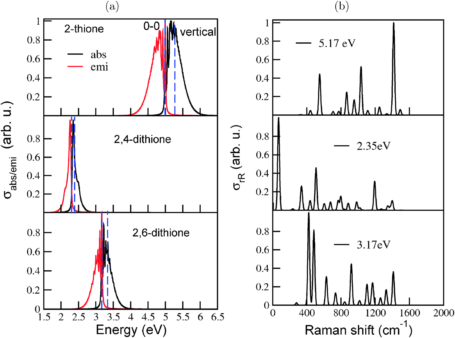 | ||
Fig. 8 (a) The vibronic absorption and emission spectra of the diamondoid thiones studied here, calculated at the B3LYP/TZVP level of theory, using the IMDHO (STA) model. From top to bottom the spectra are in the order: adamantane-2-thione, adamantane-2,4-dithione and adamantane-2,6-dithione. The dashed blue lines represent the 0–0 and vertical transition energies for all three plots. (b) The corresponding rR spectra, using the same model. The excitation energies ωL are also indicated and correspond to ΔEvibro of each molecule. Broadening parameter of Γ and  were used. For rR, resulting stick spectra were broadened by Lorentzians with FWHM of 10 cm−1. were used. For rR, resulting stick spectra were broadened by Lorentzians with FWHM of 10 cm−1. | ||
The spectra of the three molecules are energetically shifted with respect to each other, because of the different excitation energies. The absorption and emission spectra of adamantane-2,4-dithione lie in the visible energy range. The fluorescence emission spectrum of the 2,6-dithione also lies in the visible range, while the tail of the absorption spectrum extends just beyond the visible range. Adamantane-2-thione, on the other hand, absorbs and emits beyond the visible region. Vibronic finestructure is observed for adamantane-2-thione and the 2,6-dithione. The peak spacings in the absorption spectra are in the range of 520–530 cm−1 for adamantane-2-thione, whereas for the 2,6-dithione, the spacings lie in the range of 460–470 cm−1. The absorption and emission spectra of 2,4-dithione show a broad peak and a shoulder. The values of the HOMO–LUMO gaps (ΔEHL), 0–0 energies (ΔE0–0), and maxima of the absorption spectra (ΔEvibro) of the species are mentioned in Table 4, lower part. (The corresponding ΔEvert energies are shown in the upper half in bold). The IMDHO (STA) 0–0 energy (4.99 eV) of adamantane-2-thione is somewhat higher than a previously calculated value (4.66 eV) of the absorption onset (the so-called zero-phonon line) of Demján and co-workers38 using the G0W0 quasiparticle energy-correction on solutions of the Bethe–Salpeter equations (BSE)39 based on LDA wavefunctions. The experimentally reported value of the absorption onset is approximately 4.50 eV.40
Resonance Raman spectra (Fig. 8(b)) were calculated to get more insight into the normal modes facilitating the electronic transition. The spectra were calculated at excitation energies corresponding to ΔEvibro of the individual molecules. The rR spectrum of adamantane-2-thione is dominated by a combination of the CS stretching mode and C–H wagging modes, around 1420 cm−1. Lower frequency modes around 1030 cm−1 (characterized by C–C–C bending motions) and 550 cm−1 (characterized by C–S stretching and C–C–C bending motions) also show considerable intensities. The involvement of C–S stretching modes and C–C–C bending modes in rR scattering support the large increase of the CS bond length and change in C–C–C bond angles, upon electronic excitation, as mentioned earlier. The rR spectrum of the 2,4-dithione is mainly dominated by the first mode, around 67 cm−1, which is characterized by strong torsional motion of the C–C–C unit connecting the two thione groups. It is the same unit which contracted by 17° in the excited state. One of the other important modes is the one around 1190 cm−1, involving stretching of the two CS bonds. For the 2,6-dithione, normal modes involving C–C–C torsion and CS stretch are also important scatterers.
| ΔEvert | 1-X | 2-X | 1,2-X | 2,6-X |
|---|---|---|---|---|
| X = SH | 5.29 | 5.31 | 5.14 | 5.30 |
| X = OH | 6.71 | 6.76 | 6.64 | 6.69 |
| X = Br | 5.70 | 5.80 | 5.23 | 5.81 |
We note that in terms of gap reduction relative to adamantane (ΔEvert = 7.32 eV, see above), the thiols are more efficient than the bromo compounds and alcohols are least efficient. In all cases the position of the substituent for mono-substitution (1 or 2) has only a minor effect and the introduction of a second substituent has a small additional effect on the gap for 2,6-, but a slight redshift for 1,2-substitution.
For all alcohols and bromo compounds listed in the table, we also computed vibronic absorption and emission spectra using the IMDHO (STA) model. As a result (not shown), one finds pronounced vibrational finestructures for 1- and 2-alcohols and 2,6-dialcohol, while that of 1,2-dialcohol and all bromo compounds appear to be unstructured. In case of the bromo-adamantanes, absorption and emission spectra are well separated, showing Stokes shifts between 1.3 eV (2,6-dibromo) and 3.3 eV (2-bromo). In fact, for 2-bromo-adamantane, the absorption maximum is at 5.8 eV (and therefore almost equal to ΔEvert), while the emission spectrum has its maximum at around 2.5 eV (around 500 nm). Thus, emission is redshifted into the visible blue region at this level of theory. For comparison, the emission spectrum of adamantane has a maximum around 6 eV (or 200 nm), in the UV, according to a B3LYP/TZVP/IMDHOFAD calculation.18 However, although our TD-B3LYP/TZVP calculations of excited states did not converge, the C–Br bond was seen to elongate considerably (0.22 Å) during the (incomplete) optimization, hence the S1 state might actually be a dissociative state like the thiols, which is not expected to fluoresce. Experimental evidence would be very helpful.
C. C-substituted diamondoids: urotropine and related compounds
By replacing entire methylene and methine groups by hetero-atoms we can realize another class of diamondoids, called “C-substituted” in this paper.The structure of the optimized (B3LYP/TZVP) ground state of urotropine is shown in Fig. 9. Several bond lengths and bond angles have also been mentioned there.
 | ||
| Fig. 9 The B3LYP/TZVP optimized ground state geometry of urotropine. The blue balls represent the N atoms, the brown balls the C atoms and the white balls represent the H atoms. The C–N and C–H bond lengths are 1.47 Å and 1.09 Å. The C–N–C and H–C–H bond angles are around 108°, while the N–C–N bond angles are 112.4°. Bond lengths and angles involving similar atoms are equal. | ||
The C–H and C–N bond lengths are effectively unaltered in the optimized S1 state. The H–C–H bond angles increase by about 3° and some C–N–C angles increase by about 4°, while some others decrease by 2°. The N–C–N angles decrease by about 3°, but one particular N–C–N bond angle decreases to 100°, i.e., by about 12°. As seen later, this will influence the absorption and rR spectra of urotropine.
Table 6 shows selected (mostly bright) vertical excitation energies out of the first ten singlet excited states of urotropine, from the S0 state, compared to analogous values for adamantane.18
| State α | Urotropine | Adamantane | ||
|---|---|---|---|---|
| ω α (eV) | f α | ω α (eV) | f α | |
| 1 | 6.0297 | 0.0024 | 7.3223 | 0.0064 |
| 2 | 6.0300 | 0.0024 | 7.3227 | 0.0063 |
| 3 | 6.0305 | 0.0024 | 7.3232 | 0.0064 |
| ⋮ | ||||
| 9 | 6.8818 | 0.0438 | 8.4546 | 0.0000 |
| 10 | 6.8820 | 0.0438 | 8.4703 | 0.1040 |
| ΔE0–0 | 5.42 | 6.54 | ||
| ΔEHL | 6.92 | 8.15 | ||
| ΔEvibro | 5.80 | 6.84 | ||
| ΔEopt(exp.) | 5.42 | 6.49 | ||
| ΔEvibro(exp.) | ∼6.3 | 6.8 | ||
The first allowed transition is to degenerate states S1, S2 and S3 (which are only nearly degenerate in numerical practice without symmetry restrictions). These transitions are dominated by HOMO → LUMO excitations, the former being of t2 symmetry in the Td point group, the latter of a1 symmetry. The next three transitions (S4 to S6, not shown) are also three-fold degenerate but forbidden. At slightly higher energies (∼6.9 eV), further bright states follow. The behavior is qualitatively analogous to adamantane. Quantitatively, the lowest-energy absorption of urotropine is redshifted relative to adamantane, and less intense.
For both compounds, a comparison to the experimental optical gap, i.e., the onset of absorption is possible. According to Table 6, the experimental optical gaps ΔEopt(exp.) are close to the ΔE0–0 values calculated at the present level of theory. (For adamantane, this has been discussed already above.) For urotropine, a relevant comparison of the ΔE0–0 value can be made with the previously calculated absorption onset value of 5.80 eV by Demján and co-workers.38 ΔE0–0 predicts a redshift in absorption of about 1.1 eV, both in experiment14 and theory, if one considers indeed ΔE0–0 as a good measure for the optical gap.
The agreement between theory and experiment is still good but less striking when fully vibrationally resolved absorption and emission spectra are considered instead. In Fig. 10 we show S0 ↔ S1 vibronic absorption and emission spectra of urotropine, obtained on the B3LYP/TZVP/IMDHOFAD level of theory. Using the same Lorentzian broadening Γ = 200 cm−1 as in ref. 18, we find only a weak vibronic finestructure for absorption and emission of urotropine. This is contrast to pronounced finestructures found in theoretical spectra of adamantane in ref. 18 (Fig. 3 in that reference). Missing vibrational finestructure in the absorption spectrum of urotropine, but a clear finestructure for adamantane is also in full agreement with experiment.10,14 The same holds true for experimental emission spectra.10,14 A slight discrepancy between theory and experiment is found for the widths and maxima of the lowest-energy absorption and emission peaks of urotropine. For absorption, the lowest-energy band peaks at around 6.3 eV according to ref. 14, with a FWHM value of about one eV. Our absorption band is slightly narrower according to Fig. 10 (FWHM ∼ 0.6 eV), with a maximum at about 5.8 eV (Table 6). The broader experimental spectrum may result from the presence of higher states around 6.88 eV (Table 6) which have not been considered in our vibronic calculations. Similarly, our theoretical emission spectrum is redshifted by a few tenths of an eV and also narrower than the experimental one.14
 | ||
Fig. 10 The vibrationally resolved absorption and emission spectra (upper panel) for urotropine. Vertical dashed lines stand for 0–0 and vertical (for absorption) transitions, respectively. The middle panel shows the corresponding autocorrelation function for absorption. For both upper panels damping factors Γ = 200 cm−1 have been used. Resonance Raman spectra at selected excitation energies ωL are shown in the lower panel. In this case, a broadening factor  has been used and the resulting stick spectrum was broadened by normalized Lorentzians of FWHM of 10 cm−1. All calculations were at the (TD-)B3LYP/TZVP/IMDHOFAD level of theory. has been used and the resulting stick spectrum was broadened by normalized Lorentzians of FWHM of 10 cm−1. All calculations were at the (TD-)B3LYP/TZVP/IMDHOFAD level of theory. | ||
The lack of a vibrational finestructure results from the usual fact that some normal modes (e.g. modes 6 and 10, discussed later) undergo quite high displacements during the transition. Consequently, the 0–0 peak is also absent in the theoretical spectrum. The lack of vibrational finestructure in absorption is reflected in the lack of periodic recurrences in the absorption autocorrelation function (Fig. 10, middle panel), in contrast to adamantane, where clear recurrences are seen (Fig. 3(d) of ref. 18). In passing we note that using a lower broadening factor (50 cm−1) for calculating the absorption and emission spectra leads to the appearance of an extended finestructure in either case, from which little practical information about the possible contributing modes can be obtained, however. In this context, it might be relevant to mention that the choice of the broadening parameter depends essentially on the dimensionless origin shifts of the modes, which in turn, depends on the extent of geometrical distortion between the ground and excited states. Usually, for the pristine diamondoids, a FWHM of 200 cm−1 has been found to give good (compared to experiments) spectral resolution, e.g., in ref. 18. However, since most of the functionalized diamondoids involve considerably high degree of geometric distortions in the excited states, many normal modes have been found to exhibit high values of dimensionless origin-shifts, hence we had to use a lower broadening factor of FWHM = 50–100 cm−1 in most of these cases.
From the previous results, it was seen that resonance Raman spectra can provide an indication of the vibrational modes excited during electronic excitation in molecules. Therefore, the resonance Raman spectrum of urotropine was calculated and used to get a better insight into the normal modes involved in the excitation process. Fig. 10, lower panel shows the resonance Raman spectra at two different excitation energies corresponding to selected values in the resonance region. The spectra are featured by intense peaks around 510, 675, 1024, 1050, 1485 and 1500 cm−1. These peaks originate from modes 6, 10, 23, 25 and three nearly spaced modes 43, 46 and 48. The first four modes correspond to the vibrations of the six-membered rings and the N–C–N units and the last three are the various bending vibrations of the different methylene units. The intensities of the peaks corresponding to the methylene vibrations are lower than those which originate from ring torsional and N–C–N vibrational modes. The excitation of the N–C–N vibrations and some of these modes showing high values of shifts can be attributed to the change in the N–C–N bond angles during electronic excitation. This is again due to the HOMO now being centered on the nitrogen atoms. Hence, alteration of electronic structure of diamondoids can result in the alteration of their vibrational characteristics.
| Molecule | ΔEHL | ΔE0–0 | ΔEvert | ΔEvibro |
|---|---|---|---|---|
| Adamantane | 8.15 | 6.54 | 7.32 | 6.84 |
| Monooxa | 7.13 | 6.17 | 6.29 | 6.17 |
| 2,4-Dioxa | 7.44 | 6.36 | 6.60 | 6.36 |
| 2,6-Dioxa | 7.52 | 6.48 | 6.61 | 6.48 |
| 2,4,6-Trioxa | 7.83 | 6.85 | 6.92 | 6.85 |
| 2,4,10-Trioxa | 7.66 | 6.62 | 6.81 | 6.62 |
| Tetraoxa | 9.28 | 7.13 | 7.39 | 7.27 |
| Monoaza | 6.11 | 4.97 | 5.31 | 5.21 |
| Diaza | 6.05 | 4.95 | 5.23 | 5.16 |
| Triaza | 6.45 | 5.28 | 5.60 | 5.49 |
| Urotropine | 6.92 | 5.62 | 6.03 | 5.97 |
From the table we note that for aza compounds, optical gaps do not linearly decrease with the degree of N substitution. Rather, the diaza compound shows the lowest-energy absorption, followed by monoaza, triaza and urotropine. Also for oxa compounds the perhaps expected trend that more oxygens simply lead to lower absorption energies does not hold. Rather, the lowest optical gap is obtained for monooxa, followed by the di- and tri-oxas and the tetraoxa adamantane in this case. Tetraoxa adamantane is in fact an example, where the optical absorption is predicted to be blue-shifted with respect to the parent compound, adamantane. We also note that our calculated ΔE0–0 value (6.17 eV) of monooxa adamantane is in good agreement with the measured optical gap (6.18 eV) given in ref. 37.
IV. Summary and outlook
In this work, a time-dependent approach to vibronically resolved spectroscopy based on autocorrelation and cross-correlation functions was applied, along with time-dependent (linear-response) density functional theory to understand certain optical properties of electronically blended, functionalized and “doped” (or “C-substituted”) diamondoids. In particular, absorption, emission and resonance Raman spectra were computed. The Condon and harmonic approximations were used for this. The IMDHO (STA)29 and IMDHOFAD models18,25 have been used for the calculation of time-dependent correlation functions. In cases when large-amplitude motions and large displacements in excited states take place, the IMDHOFAD may be difficult to realize. Fortunately in these cases a “vertical” approach like IMDHO (STA) could also be more realistic. If one or the other approach is more appropriate, is generally still an open question.The absorption and emission spectra of the modified diamondoids are (almost all) redshifted with respect to the pristine diamondoids. The magnitude and trends of the redshift depends on the nature of the frontier orbitals which are involved in the electronic transition. This, again, depends on the nature, number and position of functional groups or substituents attached to the diamondoids. With adequate number of thione groups, for example, the absorption can be shifted to the visible region. Geometrical distortions during the electronic excitation also affect the resolution of the spectra. Important information about the vibrational normal modes playing dominant roles in the electronic excitation were extracted from the resonance Raman spectra, particularly in situations where well resolved absorption spectra could not be obtained due to significant geometrical distortions. Where comparison to experiment and previous theoretical results was possible, the present theory gave reasonable agreement. We made, however, also a large number of predictions which await experimental proof. It must be said, though, that simple explanations for observed trends are not always available. In these cases simulations are needed and therefore sufficiently accurate and at the same time sufficiently economic theoretical methods, to allow for systematic investigations of a large class of candidate materials. We believe that the present methodology is a suitable starting point.
Of course, the present methods could and should be improved. The application of more detailed basis sets and/or more accurate electronic structure methods is a worthwhile direction. Effects of anharmonicity and finite temperature might also be studied. Further, the inclusion of non-radiative transitions such as intersystem crossing by spin–orbit coupling, or internal conversion due to non-Born–Oppenheimer couplings, will be interesting to include. In this context it should be noted that the time-dependent correlation function approach may offer advantages over traditional, time-independent (Golden Rule type) approaches, too.41,42
Acknowledgements
We sincerely thank Dr Dominik Kröner, Tao Xiong (Potsdam) as well Thomas Möller and Janina Maultzsch (TU Berlin) for fruitful discussions. Financial support by the “DFG-Forschergruppe 1282” (project Sa 547/11-1) is gratefully acknowledged.References
- J. E. Dahl, S. G. Liu and R. M. K. Carlson, Science, 2003, 299, 96 CrossRef CAS PubMed
.
- P. R. Schreiner, L. V. Chernish, P. A. Gunchenko, E. Y. Tikhonchukh, H. Hausmann, M. Serafin, S. Schlecht, J. E. P. Dahl, R. M. K. Carlson and A. A. Fokin, Nature, 2011, 477, 308 CrossRef CAS PubMed
- H. Schwertfeger and P. R. Schreiner, Chem. Unserer Zeit, 2010, 44, 248 CrossRef CAS PubMed
- H. Schwertfeger, A. A. Fokin and P. R. Schreiner, Angew. Chem., Int. Ed., 2008, 47, 1022 CrossRef CAS PubMed
- W. L. Yang, J. D. Fabbri, T. M. Willey, J. R. I. Lee, J. E. Dahl, R. M. K. Carlson, P. R. Schreiner, A. A. Fokin, B. A. Tkachenko, N. A. Fokina, W. Meevasana, N. Mannella, K. Tanaka, X. J. Zhou, T. van Burren, M. A. Kelly, Z. Hussain, N. A. Melosh and Z. X. Shen, Science, 2007, 316, 1460 CrossRef CAS PubMed
- S. Roth, D. Leunberger, J. Osterwalder, J. E. Dahl, R. M. K. Carlson, B. A. Tkachenko, A. A. Fokin, P. R. Schreiner and M. Hengsberger, Chem. Phys. Lett., 2010, 495, 102 CrossRef CAS PubMed
- W. A. Clay, Z. Liu, W. Yang, J. D. Fabbri, J. E. Dahl, R. M. K. Carlson, Y. Sun, P. R. Schreiner, A. A. Fokin, B. A. Tkachenko, N. A. Fokina, P. A. Pianetta, N. Melosh and Z.-X. Shen, Nano Lett., 2009, 9, 57 CrossRef CAS PubMed
- L. Landt, K. Klünder, J. E. Dahl, R. M. K. Carlson, Th. Möller and Ch. Bostedt, Phys. Rev. Lett., 2009, 103, 047402 CrossRef
- M. Steglich, F. Husiken, J. E. Dahl, R. M. K. Carlson and Th. Henning, Astrophys. J., 2011, 729, 1 CrossRef
- R. Richter, D. Wolter, T. Zimmermann, L. Landt, A. Knecht, C. Heidrich, A. Merli, O. Dopfer, P. Reiß, A. Ehresmann, J. Petersen, J. E. Dahl, R. M. K. Carlson, C. Bostedt, T. Möller, R. Mitrić and T. Rander, Phys. Chem. Chem. Phys., 2014, 16, 3070 RSC
- R. Meinke, R. Richter, A. Merli, A. A. Fokin, T. V. Koso, V. N. Rodionov, P. R. Schreiner, C. Thomsen and J. Maultzsch, J. Chem. Phys., 2014, 140, 034309 CrossRef PubMed
- A. A. Fokin and P. R. Schreiner, Mol. Phys., 2009, 107, 823 CrossRef CAS PubMed
- A. A. Fokin, E. D. Butova, L. V. Chernish, N. A. Fokina, J. E. P. Dahl, R. M. K. Carlson and P. R. Schreiner, Org. Lett., 2007, 9, 2541 CrossRef CAS PubMed
- L. Landt, W. Kieleich, D. Wolter, M. Staiger, A. Ehresmann, Th. Möller and Ch. Bostedt, Phys. Rev. B: Condens. Matter Mater. Phys., 2009, 80, 205323 CrossRef
- L. Landt, M. Staiger, D. Wolter, K. Klünder, P. Zimmermann, T. M. Willey, T. van Bluren, D. Brehmer, P. R. Schreiner, B. A. Tkachenko, A. A. Fokin, Th. Möller and Ch. Bostedt, J. Chem. Phys., 2010, 132, 024710 CrossRef PubMed
- L. Landt, C. Bostedt, D. Wolter, Th. Möller, J. E. P. Dahl, R. M. K. Carlson, B. A. Tkachenko, A. A. Fokin, P. R. Schreiner, A. Kulesza, R. Mitrić and V. Bonačić-Koutecký, J. Chem. Phys., 2010, 132, 144305 CrossRef PubMed
- T. Rander, M. Steiger, R. Richter, T. Zimmermann, L. Landt, D. Wolter, J. E. Dahl, R. M. K. Carlson, B. A. Tkachenko, N. A. Fokina, P. R. Shreiner, T. Möller and C. Bostedt, J. Chem. Phys., 2013, 138, 024310 CrossRef PubMed
- S. Banerjee and P. Saalfrank, Phys. Chem. Chem. Phys., 2014, 16, 144 RSC
- T. Zimmermann, R. Richter, A. Knecht, A. A. Fokin, T. V. Koso, L. V. Chernish, P. A. Gunchenko, P. R. Schreiner, T. Möller and T. Rander, J. Chem. Phys., 2013, 139, 084310 CrossRef PubMed
- B. A. Tkachenko, N. A. Fokina, L. V. Chernish, J. E. P. Dahl, S. Liu, R. M. K. Carlson, A. A. Fokin and P. R. Schreiner, Org. Lett., 2006, 8, 1767 CrossRef CAS PubMed
- A. A. Fokin, T. S. Zhuk, A. E. Pashenko, P. O. Dral, P. A. Gunchenko, J. E. P. Dahl, R. M. K. Carlson, T. V. Koso, M. Serafin and P. R. Schreiner, Org. Lett., 2009, 11, 3068 CrossRef CAS PubMed
- M. Vörös, T. Demján, T. Szilvási and A. Gali, Phys. Rev. Lett., 2012, 108, 267401 CrossRef
- S. Y. Lee and E. J. Heller, J. Chem. Phys., 1979, 71, 4777 CrossRef CAS PubMed
- D. J. Tannor and E. J. Heller, J. Chem. Phys., 1982, 77, 202 CrossRef CAS PubMed
- S. Banerjee, D. Kröner and P. Saalfrank, J. Chem. Phys., 2012, 137, 22A534 CrossRef PubMed
- H. Ma, J. Liu and W. Liang, J. Chem. Theory Comput., 2012, 8, 4474 CrossRef CAS
- A. Baiardi, J. Bloino and V. Barone, J. Chem. Phys., 2014, 141, 114108 CrossRef PubMed
- J. P. Götze, B. Karasulu and W. Thiel, J. Chem. Phys., 2013, 139, 234108 CrossRef PubMed
- T. Petrenko and F. Neese, J. Chem. Phys., 2007, 127, 164319 CrossRef PubMed
- A. D. Becke, J. Chem. Phys., 1993, 98, 5648 CrossRef CAS PubMed
- C. Lee, W. Yang and R. G. Parr, Phys. Rev. B: Condens. Matter Mater. Phys., 1988, 37, 785 CrossRef CAS
- A. Schäfer, C. Huber and R. Ahlrichs, J. Chem. Phys., 1994, 100, 5829 CrossRef PubMed
-
M. J. Frisch, G. W. Trucks, H. B. Schlegel, G. E. Scuseria, M. A. Robb, J. R. Cheeseman, G. Scalmani, V. Barone, B. Mennucci, G. A. Petersson, H. Nakatsuji, M. Caricato, X. Li, H. P. Hratchian, A. F. Izmaylov, J. Bloino, G. Zheng, J. L. Sonnenberg, M. Hada, M. Ehara, K. Toyota, R. Fukuda, J. Hasegawa, M. Ishida, T. Nakajima, Y. Honda, O. Kitao, H. Nakai, T. Vreven, J. A. Montgomery, Jr., J. E. Peralta, F. Ogliaro, M. Bearpark, J. J. Heyd, E. Brothers, K. N. Kudin, V. N. Staroverov, R. Kobayashi, J. Normand, K. Raghavachari, A. Rendell, J. C. Burant, S. S. Iyengar, J. Tomasi, M. Cossi, N. Rega, J. M. Millam, M. Klene, J. E. Knox, J. B. Cross, V. Bakken, C. Adamo, J. Jaramillo, R. Gomperts, R. E. Stratmann, O. Yazyev, A. J. Austin, R. Cammi, C. Pomelli, J. W. Ochterski, R. L. Martin, K. Morokuma, V. G. Zakrzewski, G. A. Voth, P. Salvador, J. J. Dannenberg, S. Dapprich, A. D. Daniels, Ö. Farkas, J. B. Foresman, J. V. Ortiz, J. Cioslowski and D. J. Fox, Gaussian 09 (Revision A.02), Gaussian, Inc, Wallingford, CT, 2009 Search PubMed
- M. Frigo and S. G. Johnson, Proc. IEEE, 2005, 93(2), 216 CrossRef
-
F. Neese, ORCA, an ab initio, density functional and semiempirical program package, University of Bonn, Bonn, Germany, 2007 Search PubMed
- T. S. Zhuk, T. Koso, A. E. Pashenko, N. T. Hoc, V. N. Rodionov, M. Serafin, P. R. Schreiner and A. A. Fokin, J. Am. Chem. Soc., 2015, 137, 6577 CrossRef CAS PubMed
-
L. Landt, Electronic structure and optical properties of pristine and modified diamondoids, PhD thesis, Technical University of Berlin, 2010 Search PubMed
- T. Demján, M. Vörös, M. Palummo and A. Gali, J. Chem. Phys., 2014, 141, 064308 CrossRef PubMed
- G. Strinati, Phys. Rev. Lett., 1982, 49, 1519 CrossRef CAS
- K. J. Falk and R. P. Steer, Can. J. Chem., 1988, 66, 575 CrossRef CAS
- M. Etinski, J. Tatchen and C. M. Marian, J. Chem. Phys., 2011, 134, 154105 CrossRef PubMed
- Y. Niu, Q. Peng, Ch. Deng, X. Gao and Z. Shuai, J. Phys. Chem. A, 2010, 114, 7817 CrossRef CAS PubMed
| This journal is © the Owner Societies 2015 |