
[notes by Erik T.]
The following lecture is based on W. H. Zurek, “Decoherence and the transition from quantum to classical – revisited”, arXiv:quant-ph/0306072 (June 2003), an updated version of the article in Physics Today 44, 36-44 (Oct 1991).

The border between the classical and the quantum worlds. Drawing by W. H. Zurek, re-blogged in “Reading in the dark” (St. Hilda’s underground book club).
Zurek compares classical physics to quantum mechanics via the measurements in both. An example is given by a gravitational wave detector, which uses the indeterminate force on a mirror from the momentum transfer of photons. In quantum mechanics, one is in need of an amplifier to measure quantum effects because they usually occure on tiny scales: this is what N. Bohr asks for when crossing the borderline.
But this border between the macroscopic and microscopic is undefined itself. Often it is a matter of the needed precision which leads to the definition of this line. It is also related to the simplifications we make. The many worlds theory goes so far to push it back into the conciousness of the observer: to auote Zurek, this is notably an “unpleasant location to do physics”.
Decoherence is the loss of the ability to interfere. It happens because of the exchange of information and energy between a system and its environment. Zurek especially considers quantum-chaotic systems, so first of all we need to define what a chaotic system is. A chaotic system is characterised by its strong dependence on initial conditions and on perturbations. An example for this is the “baker’s map” illustrated below: an area gets stretched and compressed and then folded back together. This leads, after a few iterations, to a complete disruption of initial structures.

Visualization of the baker’s map, inspired from a figure in S. Strogatz, Nonlinear Dynamics and Chaos: With Applications to Physics, Biology, Chemistry, and Engineering (Westview Press 1994).
For a quantum system this means that an initial distribution in phase-space gets folded and stretched such that after a certain time it exhibits fine structures. The Wigner function 
Note: this way of thinking about quantum chaos cannot be fully compared to classical mechanics, because chaos doesn’t exist in the typical sense here. If two wave functions overlap, they will always overlap, since the unitary Hamiltonian conserves such geometric properties.
Assume 

We can now look at the friction and the resulting diffusion by using the differential equation for Brownian motion. It has the same structure as the equation for heat diffusion:
So by plugging in 

and this can easily be solved as 


where 

For the system to be at equilibrium, both processes have to be equal, so

But in equilibrium, we also have

where 
and for 


Schrödinger’s cat and Wigner’s infinite regression
Let’s take a step back and look at Schrödingers cat again, where nuclear decay determines the state of the cat. The atom is in a superposition of states of being decayed and not being decayed, the Geiger counter is also in a superposition, namely of detecting an event and not detecting one and so on. Now where do we draw the line of thinking about superposition, the cat? Or the observer? Or even the Universe? This is Wigner’s infinite regression. It seems obvious, that a good theory needs to break up this line of reasoning somewhere. So it has to properly define the border between micro and macro.
Example: Schrödinger’s cat
The cat is seemingly in a superposition of states 
Example: oscillator at temperature
Hamiltonian

spring constant and oscillator frequency

Wigner function of thermal equilibrium state
![\displaystyle W_T(x, p) = \frac{1}{Z} \exp\left[-\frac{2 H}{\hbar \omega \coth \left(\frac{\hbar \omega}{2 k_B T}\right)} \right]](https://s0.wp.com/latex.php?latex=%5Cdisplaystyle+W_T%28x%2C+p%29+%3D+%5Cfrac%7B1%7D%7BZ%7D+%5Cexp%5Cleft%5B-%5Cfrac%7B2+H%7D%7B%5Chbar+%5Comega+%5Ccoth+%5Cleft%28%5Cfrac%7B%5Chbar+%5Comega%7D%7B2+k_B+T%7D%5Cright%29%7D+%5Cright%5D+&bg=ffffff&fg=000&s=0&c=20201002)
So here we have an uncertainty product
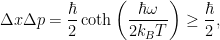
larger than the minimum allowed by the Heisenberg uncertainty principle.
3 Replies to “Decoherence”